8.3. Random Forest Classification

8.3.1. Random Forest Tutorial Aims:

• Random Forest classification with scikit-learn

• How random forests work

• How to use them for regression

• How to evaluate their performance (& tune Hyper-parameters)

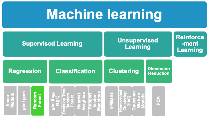
8.3.2. What is a Random Forest?

• RF are built by combining mulitple DT (ensemble of decision trees to predict target variables)

• RFs combine simplicity of DTs with flexiblity –> therefore improved accuracy

• RFs are for supervised machine learning, where there is a labeled target variable.

• RFs can be used for solving regression (numeric target variable) and classification (categorical target variable) problems.

• RFs are an ensemble method, meaning they combine predictions from other models.

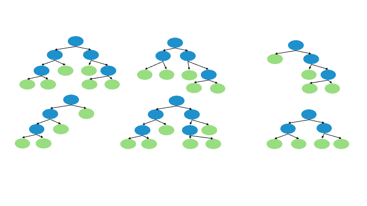
8.3.3. How does it work?

A Random forest regression model combines multiple decision trees to create a single model. Each tree in the forest builds from a different subset of the data and makes its own independent prediction. The final prediction for input is based on the average or weighted average of all the individual trees’ predictions.

Read here more on the theory.

Nice introductory video

8.3.3.1. Step by Step:

• 1. Create a “bootstrapped” dataset.

  • Randomly select samples from the original dataset. The same sample can be picked more than once.

• 2. Create a decision tree using that “bootstrapped” dataset. But only use a random subset of variables (columns) at each step.

• 3. Go back to 1 and repeat. Make a new bootstrapped dataset and built a tree on a subset of variables, resulting in a variaty of trees.

• 4. Running new data down all of the trees, results in a “vote” for the target variable.

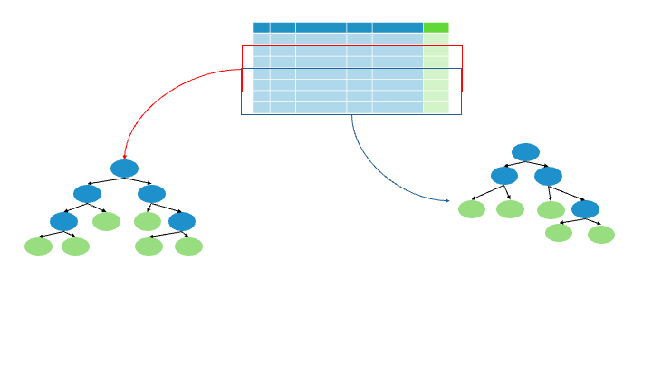
Terminology:

Bagging: Bootstrapping + Using the Aggregate to make a decision

8.3.4. Evaluation

• 1/3 of the data does not end up in the “bootstrapped” dataset = Out-Of-Bag Dataset

• Evaluate all trees with the Out-Of-Bag Dataset,

• proportion of incorrectly classified samples = Out-Of-Bag Error , OOB

8.3.5. Example: Building a Random Forest

Now, we will built a Random Forest by revisiting the example, we introduced in the decision tree script. Split data into target and features and perform the train-test-split (70-30).

%load_ext lab_black

# Load libraries
import pandas as pd
import numpy as np
import matplotlib.pyplot as plt
import seaborn as sns

from sklearn.tree import DecisionTreeClassifier  # Import Decision Tree Classifier
from sklearn.model_selection import train_test_split  # Import train_test_split function
from sklearn import (
    metrics,
)  # Import scikit-learn metrics module for accuracy calculation
from sklearn import tree

# load data

data = {
    "clouds": [1, 0, 1, 0, 0, 0, 1],
    "temp": [10, 20, -3, -5, 25, 10, 30],
    "rain": [1, 0, 0, 0, 0, 0, 1],
}
df = pd.DataFrame.from_dict(data)
df

	clouds	temp	rain
0	1	10	1
1	0	20	0
2	1	-3	0
3	0	-5	0
4	0	25	0
5	0	10	0
6	1	30	1

#### your code here ####

8.3.5.1. solution

# split dataset in features and target variable
feature_cols = ["clouds", "temp"]
X = df[feature_cols]  # Features
y = df.rain  # Target variable

# Split dataset into training set and test set
X_train, X_test, y_train, y_test = train_test_split(
    X, y, test_size=0.3, random_state=1
)  # 70% training and 30% test

8.3.6. Model

Build the Random Forest Classfier an fit the model

# Importieren von Modulen/Bibliotheken
from sklearn.ensemble import RandomForestClassifier
from sklearn.metrics import mean_squared_error

# Initialwert und Anzahl der Bäume für den Random Forest festlegen
seed = 196
n_estimators = 1000

# RandomForest erstellen, X und y definieren und Modell trainieren
model = RandomForestClassifier(
    n_estimators=n_estimators,
    random_state=seed,
    max_features=1.0,
    min_samples_split=2,
    min_samples_leaf=1,
    max_depth=None,
    oob_score=True,
)
model.fit(X_train, y_train)

RandomForestClassifier(max_features=1.0, n_estimators=1000, oob_score=True,
                       random_state=196)

In a Jupyter environment, please rerun this cell to show the HTML representation or trust the notebook.
On GitHub, the HTML representation is unable to render, please try loading this page with nbviewer.org.

Exercise: Evaluate the Random Forest

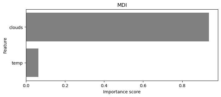
Calculte the RMSE, OOB Score and plot the feature importance. Which one is more important to predict rain?

#### your code here ####

8.3.6.1. solution

# Mittelwert der quadrierten Residuen und erklärte Varianz ausgeben lassen
print(f"Mean of squared residuals: {model.score(X, y)}")
print(f"% Var explained: {model.score(X, y) * 100}")


print(f"% OOB score: {1 - model.oob_score_}")

Mean of squared residuals: 0.8571428571428571
% Var explained: 85.71428571428571
% OOB score: 0.25

# Statistiken über das Modell ausgeben lassen und die 10 wichtigsten Variablen extrahieren
stats = model.get_params()
feature_importance = model.feature_importances_
features = X.columns
var_imp_df = pd.DataFrame({"Feature": features, "Importance": feature_importance})
var_imp_df = var_imp_df.sort_values(by="Importance", ascending=False).head(54)
var_imp_10 = var_imp_df.head(10)

# Plotten der wichtigsten Variablen
plt.figure(figsize=(8, 3))
sns.barplot(x="Importance", y="Feature", data=var_imp_10, color="gray")
plt.title("MDI")
plt.xlabel("Importance score")
plt.ylabel("Feature")

plt.show()

Sample locations

The data set and further information about the sampling process can be found here.

Let us take a closer look at the data:

# Importieren der pandas- und requests-Bibliothek sowie des StringIO-Moduls
import pandas as pd
import requests
from io import StringIO

# Daten über URL einlesen
url = "https://doi.pangaea.de/10.1594/PANGAEA.944811?format=textfile"

response = requests.get(url)
IsoW06 = pd.read_csv(StringIO(response.text), sep = '\t', skiprows = 267, header = 1, encoding = "UTF-8", 
                     engine = 'python', on_bad_lines = 'skip')

# Anzeigen der ersten 6 Dateneinträge
IsoW06.head(6)

	Event	Sample ID	Latitude	Longitude	Date/Time	Samp type	Sample comment	δ18O H2O [‰ SMOW]	δD H2O [‰ SMOW]	δ18O H2O std dev [±]	δD H2O std dev [±]
0	WaterSA_SLW1	SLW1	-33.88917	18.96917	2016-08-29	River	River at Pniel	-3.54	-14.50	0.09	0.64
1	WaterSA_SLW2	SLW2	-33.87800	19.03517	2016-08-29	River	River Berg; abundant with insect larvae; dam u...	-3.33	-13.62	0.09	0.45
2	WaterSA_SLW3	SLW3	-33.93667	19.17000	2016-08-29	River	Minor waterfall; iron rich	-4.44	-22.33	0.04	0.59
3	WaterSA_SLW4	SLW4	-33.69350	19.32483	2016-08-29	River	River; abundant with insect larvae	-4.28	-22.70	0.07	0.30
4	WaterSA_SLW5	SLW5	-33.54333	19.20733	2016-08-29	River	River Bree	-4.09	-18.99	0.04	0.34
5	WaterSA_SLW6	SLW6	-33.33367	19.87767	2016-08-30	Lake	Reservoir lake; under almost natural condition...	-2.59	-18.59	0.10	0.29

The data set contains 188 samples and the following 11 variables: Event, Sample ID, Latitude, Longitude, Date/Time, Samp type, Sample comment, δ18O H2O [‰ SMOW], δD H2O [‰ SMOW], δ18O H2O std dev [±], δD H2O std dev [±]. The isotope ratios are expressed in the conventional delta notation (δ18O, δ2H) in per mil (‰) relative to VSMOW (Vienna Standard Mean Ocean Water.

8.3.6.2. Ressources for this script:

• Koehrsen 2010

from IPython.display import IFrame

IFrame(
    src="../../citations/citation_marie.html",
    width=900,
    height=200,
)