3.4. Additional Exercises IV - Feature Scales

# First, let's import all the needed libraries.
import numpy as np
import math
import pandas as pd
import matplotlib.pyplot as plt

\[\log {_2}{64} = 6 \]

\[\log {_{10}}{1000} = 3 \]

\[\log {_3}{27} = 3 \]

\[9^{0.5} = 3\]

\[64^\frac{1}{6} = 2\]

\[8^0 = 1\]

\[\log{\frac{a}{b}} \]

\[2 * \log{{b}} \]

\[\frac{1}{3} \]

3.4.1. 1. An Arbitrary Example

Inspired by Soga FU Berlin

Take a closer look at this hypothetical example of a survey among students. In this survey, students were asked how important they consider practice exercises to be for their own learning success. 1 is not important at all and 10 is extremely important. A total of 254 students were surveyed. After the analysis, the following results are presented in %:

## poll results as dictionary
poll = {
    "score": np.arange(1, 11, 1),
    "percent": [1, 0.2, 0, 3, 7, 8, 20, 32, 16.4, 12],
}

## convert to pandas
poll = pd.DataFrame(poll)
print(poll)

   score  percent
0      1      1.0
1      2      0.2
2      3      0.0
3      4      3.0
4      5      7.0
5      6      8.0
6      7     20.0
7      8     32.0
8      9     16.4
9     10     12.0

3.4.1.1. 1.1. Calculate the mean and Plotting

Plot the data as a bar plot and calculate the mean of the survey results. Do you notice anything unusual about the data and the statistical parameters? Reconstruct the data and calculate the mean!

3.4.1.1.1. solution

## reconstructing the data
n = 254
absolute_votes = round(
    poll.percent / 100 * n
)  # convert percentage to abosulte numbers and round to have full people --> induces uncertainty

## no a small loop
poll_raw = []
for x, c in zip(poll.score, absolute_votes):
    interim = np.repeat(x, c)
    poll_raw.extend(interim)
poll_raw = np.array(poll_raw)

# get the mean

mean = np.mean(poll_raw)
mean

7.5984251968503935

We have a second option here to calculate the mean:

1. The weighted mean (since we are dealing with percentage data here). $\( \bar x_w = \frac{\sum_{i=1}^n w_ix_i }{\sum_{i=1}^n w_i} \)$

wi = weights (percentages) , xi = scores

weighted_mean = sum(poll["score"] * poll["percent"]) / sum(poll["percent"])
weighted_mean

## is slightly different because of our prior rounding --> but very similar

7.630522088353414

plt.bar(poll.score, poll.percent, color="green", edgecolor="black")
plt.axvline(mean, color="red")  ## add the mean to the plot
plt.show()

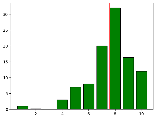
Have you noticed it already? Lets have a closer look, since the figure contains a lot of information:

1. The absolute majority voted on the upper part of the scale

2. Only 3 individual voted “not important at all” (0 or 1)

3. Nearly one third voted for the third highest value (8)

4. 60% voted for levels ≥8

5. A “Score” reports a value of ~7.6 which is below 8 !!

Why is the mean as measure of central tendency smaller than the values of 60% of the voters?

We can exclude several phenomena for this weird poll outcome as shown here

What is the reason?

3.4.1.2. 1.2. Noticing the bounds and resolving them

Calcuting the arithmetic mean seems to be unsufficient here, but why? Lets think about the margins the people were allowed to vote in between. What the upper and the lower bound ?

Ok Ok, may be a bit trivial here, but:

Choosing one number is related to two information:

• the distance to the lower margin and (0)

• the distance to the upper margin! (10)

Both distances are sum up to the width of the interval. Hereby, neither the margins themselves nor the width of the interval are important. Only the amount of possible eligible numbers influences the resolution of the measure.

Thus, any number reflects a relative measure towards the margins and can therefore be transformed to a standard interval as [0,1] or [0,100%].

However, for a meaningful examination of the constraint values, we should focus on the relation of both equal important measures, e.g. for [0,1].

In our case, we applay logistic transformation resp. logit, as we already saw in the seminar (sea ice example):

\[ x\to x'=log\left( \frac{x}{1-x}\right)\]

The back transformation is the “logistic” function resp. inverse logit: $\( x' \to x=\frac{e^{x'}}{1+e^{x'}}\)$

Nice, we just follow our recipe then! Apply the transformation to our poll data!

3.4.1.2.1. 1.2.1. Min-Max-Scaling

But before we start we have to enlarge our interval by a small constant c to avoid zeros when the original margin has been voted. Set a small constant c for min-max-Transformation into the simplex:

The min-max scaling

\[x'=\frac{x-x_{min}}{x_{max}-x_{min}}\]

transforms the data into the range \([0,1]\). We want to avoid getting values with 0, because in the second step we need the logarithm of the values. Therefore, we use slightly larger boundary values \(x_{min}-1\) and \(x_{max}+1\). Thus

\[x'=\frac{x-x_{min}+1}{x_{max}-x_{min}+2\, .}\]

3.4.1.2.2. solution

# set a small constant c to avoid zeros:
c = 0.01
# min-max-transformation
min_max_poll = (poll_raw - (1 - c)) / (10 - 1 + 2 * c)

3.4.1.2.3. 1.2.2. Perform a logistic transformation on x′∈]0,1[ℝ

\[ x\to x'=log\left( \frac{x}{1-x}\right)\]

Perform a logistic transformation on x′∈]0,1[ℝ

Plot the data again as histogram, how does the distribution look now?

Then we can calculate the desired parameters agaiin (e.g., mean, median …)!

3.4.1.2.4. solution

# logistic transformation
poll_log = np.log(min_max_poll / (1 - min_max_poll))

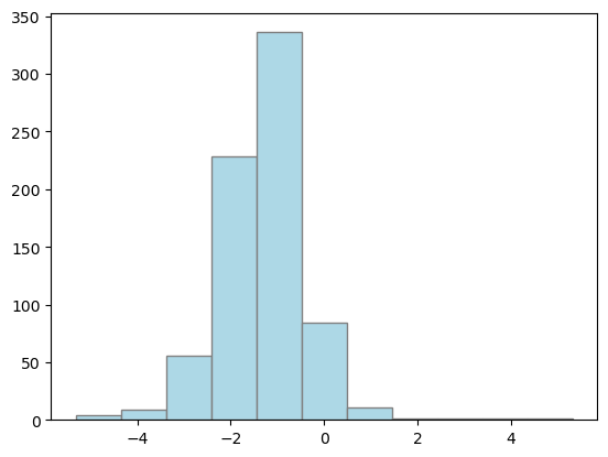
## lets plot again
plt.hist(poll_log)
plt.show()

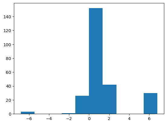
Looks alot less skewed!

lets calculate the mean again:

m_log = np.mean(poll_log)
med_log = np.median(poll_log)

## and in addition the confidence bounds, this is just an extra here !
CI_low = m_log - np.std(poll_log) / np.sqrt(len(poll_log))
CI_up = m_log + np.std(poll_log) / np.sqrt(len(poll_log))

3.4.1.3. 1.3. Backtransform

Transform these paramters back by applying exponential function. Have we resolved this issue now?

3.4.1.3.1. solution

corrected_mean = (1 - c) + (9 + 2 * c) * np.exp(m_log) / (1 + np.exp(m_log))
corrected_median = (1 - c) + (9 + 2 * c) * np.exp(med_log) / (1 + np.exp(med_log))
corrected_CI_low = (1 - c) + (9 + 2 * c) * np.exp(CI_low) / (1 + np.exp(CI_low))
corrected_CI_up = (1 - c) + (9 + 2 * c) * np.exp(CI_up) / (1 + np.exp(CI_up))


print(
    f"corrected mean =",
    {round(corrected_mean, 2)},
    "corrected median=",
    {round(corrected_median, 2)},
    "confidence interval=[",
    {round(corrected_CI_low, 2)},
    ",",
    {round(corrected_CI_up, 2)},
    "]",
)

corrected mean = {8.46} corrected median= {8.0} confidence interval=[ {8.28} , {8.63} ]

We not only get a reasonable mean, the confidence bounds are asymmetric as it should be for skewed distributions. Furthermore, these transformations have not influenced the median! (As it should be!)

3.4.2. 2. Working with real Data

3.4.2.1. DWD data

We begin by loading the meteorological data set from the Deutscher Wetterdienst DWD (German Weather Service) Open Climate Data Center . You find a documentation of this data in german and english.

We will reuse this data from the prior exercise.

dahlem_clim = pd.read_csv(
    "https://userpage.fu-berlin.de/soga/data/raw-data/NS_TS_Dahlem.txt", sep=";"
)
dahlem_clim.head(10)

	STATIONS_ID	MESS_DATUM_BEGINN	MESS_DATUM_ENDE	QN_4	MO_N	MO_TT	MO_TX	MO_TN	MO_FK	MX_TX	MX_FX	MX_TN	MO_SD_S	QN_6	MO_RR	MX_RS	eor
0	403	17190101	17190131	5	-999.0	2.8	-999.0	-999.0	-999.0	-999.0	-999.0	-999.0	-999.0	-999	-999.0	-999.0	eor
1	403	17190201	17190228	5	-999.0	1.1	-999.0	-999.0	-999.0	-999.0	-999.0	-999.0	-999.0	-999	-999.0	-999.0	eor
2	403	17190301	17190331	5	-999.0	5.2	-999.0	-999.0	-999.0	-999.0	-999.0	-999.0	-999.0	-999	-999.0	-999.0	eor
3	403	17190401	17190430	5	-999.0	9.0	-999.0	-999.0	-999.0	-999.0	-999.0	-999.0	-999.0	-999	-999.0	-999.0	eor
4	403	17190501	17190531	5	-999.0	15.1	-999.0	-999.0	-999.0	-999.0	-999.0	-999.0	-999.0	-999	-999.0	-999.0	eor
5	403	17190601	17190630	5	-999.0	19.0	-999.0	-999.0	-999.0	-999.0	-999.0	-999.0	-999.0	-999	-999.0	-999.0	eor
6	403	17190701	17190731	5	-999.0	21.4	-999.0	-999.0	-999.0	-999.0	-999.0	-999.0	-999.0	-999	-999.0	-999.0	eor
7	403	17190801	17190831	5	-999.0	18.8	-999.0	-999.0	-999.0	-999.0	-999.0	-999.0	-999.0	-999	-999.0	-999.0	eor
8	403	17190901	17190930	5	-999.0	13.9	-999.0	-999.0	-999.0	-999.0	-999.0	-999.0	-999.0	-999	-999.0	-999.0	eor
9	403	17191001	17191031	5	-999.0	9.0	-999.0	-999.0	-999.0	-999.0	-999.0	-999.0	-999.0	-999	-999.0	-999.0	eor

3.4.2.2. 2.1. Subsetting the data frame

First, we want to subset the entire dataset.

We only want to keep data from 1961 to today. Subset the entire dataset (not only 1 column as we saw in the seminar)!

How many rows has the dataframe now?

3.4.2.2.1. solution

## you could do e.g.,:
dahlem_clim = dahlem_clim.loc[dahlem_clim["MESS_DATUM_BEGINN"] >= 19610101]
dahlem_clim.head(10)

	STATIONS_ID	MESS_DATUM_BEGINN	MESS_DATUM_ENDE	QN_4	MO_N	MO_TT	MO_TX	MO_TN	MO_FK	MX_TX	MX_FX	MX_TN	MO_SD_S	QN_6	MO_RR	MX_RS	eor
2778	403	19610101	19610131	5	5.01	-1.02	1.31	-3.88	2.63	7.8	-999.0	-16.2	71.5	5	50.4	7.4	eor
2779	403	19610201	19610228	5	6.12	4.66	7.98	1.56	2.56	15.5	-999.0	-4.7	61.4	5	41.9	7.6	eor
2780	403	19610301	19610331	5	5.58	6.79	10.79	3.15	3.02	19.4	-999.0	-3.7	124.1	5	52.9	18.6	eor
2781	403	19610401	19610430	5	4.88	11.38	16.61	6.24	2.40	26.1	-999.0	-0.9	192.7	5	55.7	13.3	eor
2782	403	19610501	19610531	5	6.11	11.23	15.54	7.18	2.29	23.8	-999.0	3.0	132.8	5	120.1	26.7	eor
2783	403	19610601	19610630	5	4.39	17.73	23.18	11.47	2.12	30.4	-999.0	5.5	273.4	5	48.3	13.4	eor
2784	403	19610701	19610731	5	5.79	16.16	20.88	12.14	2.49	33.0	-999.0	8.8	143.2	5	72.6	13.2	eor
2785	403	19610801	19610831	5	5.34	15.97	21.20	11.40	2.40	28.5	-999.0	8.0	169.7	5	43.0	10.3	eor
2786	403	19610901	19610930	5	3.48	15.95	22.00	11.06	2.11	30.0	-999.0	4.4	201.7	5	35.5	12.1	eor
2787	403	19611001	19611031	5	4.77	11.10	15.54	7.26	2.39	22.3	-999.0	3.3	136.8	5	35.7	16.4	eor

dahlem_clim.shape[0]  # number of rows

732

3.4.2.3. 2.2. Checking for Normality

We want to work with the precipitation sum per month in mm now. Its written the the MO_RR column. Plot the distribution as histogram or density plot and a QQ-plot to visually check for normal distribution (solution the same as the prior exercise). Do mean and standard deviation violate the 3-sigma rule?

3.4.2.3.1. solution

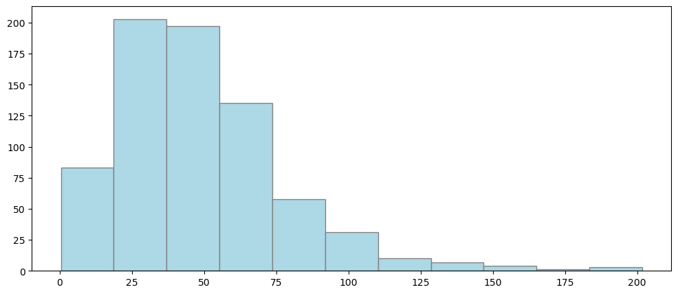
plt.figure(figsize=(12, 5))
plt.hist(dahlem_clim.MO_RR, bins="sturges", color="lightblue", edgecolor="grey")

plt.show()

import statsmodels.api as sm

plt.figure(figsize=(12, 5))
sm.qqplot(dahlem_clim.MO_RR, line="r")

plt.show()

<Figure size 1200x500 with 0 Axes>

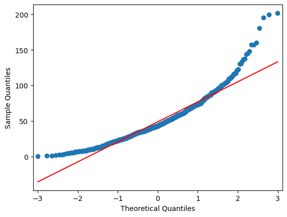
Ok, looks skewed! There seems to be no normal distribution…..and 3-sigma is also not fulfilled:

np.mean(dahlem_clim.MO_RR), np.std(dahlem_clim.MO_RR)

(48.77950819672131, 29.232662243364572)

np.median(dahlem_clim.MO_RR)

43.150000000000006

3.4.2.4. 2.3. Transforming the Data

In the prior exercise we saw that the precipitation data is not normally distributed and that calculating the mean and standard deviation violates the 3-sigma rule! Apply the “recipe” we saw in the seminar for double bounded scales (same as exercise above):

1. scale your variable for min-max and log transform your variable

2. Calculate statistics, Plot histogram of log-transformed data (mean and std)

3. Backtransform using exp()

How about the 3-sigma rule now?

3.4.2.4.1. solution

1. Min-Max Scaling

dahlem_MO_RR_transfo = (
    dahlem_clim.MO_RR.copy()
)  # set an equivalent copy to perform the feature scales transformation

xmin = dahlem_MO_RR_transfo.min()
xmax = dahlem_MO_RR_transfo.max()

# transform each column by its indiv. min/max
dahlem_MO_RR_transfo = (dahlem_MO_RR_transfo - xmin + 1) / (xmax - xmin + 2)

2. Perform a logistic transformation on x′∈]0,1[ℝ

# Perform a logistic transformation on x′∈]0,1[ℝ

dahlem_MO_RR_transfo = np.log(dahlem_MO_RR_transfo / (1 - dahlem_MO_RR_transfo))

3. Histogram Plotting

## lets plot again
plt.hist(dahlem_MO_RR_transfo, bins="sturges", color="lightblue", edgecolor="grey")
plt.show()

4. Calculate statistics (e.g., mean and confidence bounds…)

m_log = np.mean(dahlem_MO_RR_transfo)
med_log = np.median(dahlem_MO_RR_transfo)

## and in addition the confidence bounds, this is just an extra here !
CI_low = m_log - np.std(dahlem_MO_RR_transfo) / np.sqrt(len(dahlem_MO_RR_transfo))
CI_up = m_log + np.std(dahlem_MO_RR_transfo) / np.sqrt(len(dahlem_MO_RR_transfo))

5. Backtransform: Transform these parameters back by applying exponential function. Have we resolved this issue now?

# backtransform
## reverse min max und perform exp()

corrected_mean = (xmin - 1) + (xmax - xmin + 2) * (np.exp(m_log) / (1 + np.exp(m_log)))
corrected_median = (xmin - 1) + (xmax - xmin + 2) * (
    np.exp(med_log) / (1 + np.exp(med_log))
)
corrected_CI_low = np.exp(CI_low) / (1 + np.exp(CI_low)) * (xmax - xmin + 2) - 1 + xmin
corrected_CI_up = np.exp(CI_up) / (1 + np.exp(CI_up)) * (xmax - xmin + 2) - 1 + xmin


print(
    f"corrected mean =",
    {round(corrected_mean, 2)},
    "corrected median=",
    {round(corrected_median, 2)},
    "confidence interval=[",
    {round(corrected_CI_low, 2)},
    ",",
    {round(corrected_CI_up, 2)},
    "]",
)

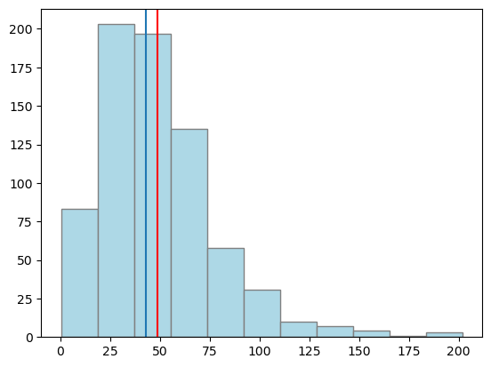
corrected mean = {43.06} corrected median= {43.15} confidence interval=[ {41.89} , {44.25} ]

## lets plot again
dahlem_MO_RR_back_transfo = (xmin - 1) + (xmax - xmin + 2) * (
    np.exp(dahlem_MO_RR_transfo) / (1 + np.exp(dahlem_MO_RR_transfo))
)


plt.hist(dahlem_MO_RR_back_transfo, bins="sturges", color="lightblue", edgecolor="grey")
plt.axvline(np.mean(dahlem_clim.MO_RR), color="red")
plt.axvline(corrected_mean)
plt.show()

from IPython.display import IFrame

IFrame(
    src="../../../citation_Marie.html",
    width=900,
    height=200,
)