2.3. Additional Exercises III - The Normal distribution#
2.3.1. Exercise 1: Recall Statistics#
In order to apply AI algorithms, write codes and evaluate large data sets, we need some statistics.
Recall in groups the following topics:
What is a normal distribution? What is a standard deviation, the variance, confidence intervalls?
What kind of means are there?
What is the central limit theorem
What is the law of large numbers?
What is linear regression?
What is logistische Regression?
What is a general linear model (GLM)?
What is a Poisson distribution?
2.3.2. Exercise 2: Checking for Normal Distribution#
2.3.2.1. DWD data#
We begin by loading the meteorological data set from the Deutscher Wetterdienst DWD (German Weather Service) Open Climate Data Center . You find a documentation of this data in german and english.
# First, let's import all the needed libraries.
import numpy as np
import pandas as pd
import matplotlib.pyplot as plt
import seaborn as sns
dahlem_clim = pd.read_csv(
    "https://userpage.fu-berlin.de/soga/data/raw-data/NS_TS_Dahlem.txt", sep=";"
)
dahlem_clim.head(10)
| STATIONS_ID | MESS_DATUM_BEGINN | MESS_DATUM_ENDE | QN_4 | MO_N | MO_TT | MO_TX | MO_TN | MO_FK | MX_TX | MX_FX | MX_TN | MO_SD_S | QN_6 | MO_RR | MX_RS | eor | |
|---|---|---|---|---|---|---|---|---|---|---|---|---|---|---|---|---|---|
| 0 | 403 | 17190101 | 17190131 | 5 | -999.0 | 2.8 | -999.0 | -999.0 | -999.0 | -999.0 | -999.0 | -999.0 | -999.0 | -999 | -999.0 | -999.0 | eor |
| 1 | 403 | 17190201 | 17190228 | 5 | -999.0 | 1.1 | -999.0 | -999.0 | -999.0 | -999.0 | -999.0 | -999.0 | -999.0 | -999 | -999.0 | -999.0 | eor |
| 2 | 403 | 17190301 | 17190331 | 5 | -999.0 | 5.2 | -999.0 | -999.0 | -999.0 | -999.0 | -999.0 | -999.0 | -999.0 | -999 | -999.0 | -999.0 | eor |
| 3 | 403 | 17190401 | 17190430 | 5 | -999.0 | 9.0 | -999.0 | -999.0 | -999.0 | -999.0 | -999.0 | -999.0 | -999.0 | -999 | -999.0 | -999.0 | eor |
| 4 | 403 | 17190501 | 17190531 | 5 | -999.0 | 15.1 | -999.0 | -999.0 | -999.0 | -999.0 | -999.0 | -999.0 | -999.0 | -999 | -999.0 | -999.0 | eor |
| 5 | 403 | 17190601 | 17190630 | 5 | -999.0 | 19.0 | -999.0 | -999.0 | -999.0 | -999.0 | -999.0 | -999.0 | -999.0 | -999 | -999.0 | -999.0 | eor |
| 6 | 403 | 17190701 | 17190731 | 5 | -999.0 | 21.4 | -999.0 | -999.0 | -999.0 | -999.0 | -999.0 | -999.0 | -999.0 | -999 | -999.0 | -999.0 | eor |
| 7 | 403 | 17190801 | 17190831 | 5 | -999.0 | 18.8 | -999.0 | -999.0 | -999.0 | -999.0 | -999.0 | -999.0 | -999.0 | -999 | -999.0 | -999.0 | eor |
| 8 | 403 | 17190901 | 17190930 | 5 | -999.0 | 13.9 | -999.0 | -999.0 | -999.0 | -999.0 | -999.0 | -999.0 | -999.0 | -999 | -999.0 | -999.0 | eor |
| 9 | 403 | 17191001 | 17191031 | 5 | -999.0 | 9.0 | -999.0 | -999.0 | -999.0 | -999.0 | -999.0 | -999.0 | -999.0 | -999 | -999.0 | -999.0 | eor |
2.3.3. Exercise 2A: Subsetting the data frame#
First, we want to subset the entire dataset.
We only want to keep data from 1961 to day. Subset the entire dataset (not only 1 column as we saw in the seminar)! hwo many rows has the dataframe now?
### your code here ###
2.3.3.1. solution#
## you could do e.g.,:
dahlem_clim = dahlem_clim.loc[dahlem_clim["MESS_DATUM_BEGINN"] >= 19610101]
dahlem_clim.head(10)
| STATIONS_ID | MESS_DATUM_BEGINN | MESS_DATUM_ENDE | QN_4 | MO_N | MO_TT | MO_TX | MO_TN | MO_FK | MX_TX | MX_FX | MX_TN | MO_SD_S | QN_6 | MO_RR | MX_RS | eor | |
|---|---|---|---|---|---|---|---|---|---|---|---|---|---|---|---|---|---|
| 2778 | 403 | 19610101 | 19610131 | 5 | 5.01 | -1.02 | 1.31 | -3.88 | 2.63 | 7.8 | -999.0 | -16.2 | 71.5 | 5 | 50.4 | 7.4 | eor |
| 2779 | 403 | 19610201 | 19610228 | 5 | 6.12 | 4.66 | 7.98 | 1.56 | 2.56 | 15.5 | -999.0 | -4.7 | 61.4 | 5 | 41.9 | 7.6 | eor |
| 2780 | 403 | 19610301 | 19610331 | 5 | 5.58 | 6.79 | 10.79 | 3.15 | 3.02 | 19.4 | -999.0 | -3.7 | 124.1 | 5 | 52.9 | 18.6 | eor |
| 2781 | 403 | 19610401 | 19610430 | 5 | 4.88 | 11.38 | 16.61 | 6.24 | 2.40 | 26.1 | -999.0 | -0.9 | 192.7 | 5 | 55.7 | 13.3 | eor |
| 2782 | 403 | 19610501 | 19610531 | 5 | 6.11 | 11.23 | 15.54 | 7.18 | 2.29 | 23.8 | -999.0 | 3.0 | 132.8 | 5 | 120.1 | 26.7 | eor |
| 2783 | 403 | 19610601 | 19610630 | 5 | 4.39 | 17.73 | 23.18 | 11.47 | 2.12 | 30.4 | -999.0 | 5.5 | 273.4 | 5 | 48.3 | 13.4 | eor |
| 2784 | 403 | 19610701 | 19610731 | 5 | 5.79 | 16.16 | 20.88 | 12.14 | 2.49 | 33.0 | -999.0 | 8.8 | 143.2 | 5 | 72.6 | 13.2 | eor |
| 2785 | 403 | 19610801 | 19610831 | 5 | 5.34 | 15.97 | 21.20 | 11.40 | 2.40 | 28.5 | -999.0 | 8.0 | 169.7 | 5 | 43.0 | 10.3 | eor |
| 2786 | 403 | 19610901 | 19610930 | 5 | 3.48 | 15.95 | 22.00 | 11.06 | 2.11 | 30.0 | -999.0 | 4.4 | 201.7 | 5 | 35.5 | 12.1 | eor |
| 2787 | 403 | 19611001 | 19611031 | 5 | 4.77 | 11.10 | 15.54 | 7.26 | 2.39 | 22.3 | -999.0 | 3.3 | 136.8 | 5 | 35.7 | 16.4 | eor |
dahlem_clim.shape[0] # number of rows
732
2.3.4. Exercise 2B: Checking the mean and standard deviation for this subset#
Calculate the mean and standard deviation for the monthly mean temperature! Doe they violate the three sigma rule? plot the distriubtion as histogram and density plot.
### your code here ###
2.3.4.1. solution#
np.mean(dahlem_clim.MO_TT), np.std(
    dahlem_clim.MO_TT
)  ## Yes it violates the 3 sigma rule!
(9.404439890710382, 6.846380527375167)
plt.figure(figsize=(10, 5))
plt.hist(dahlem_clim.MO_TT, bins="sturges", color="lightblue", edgecolor="grey")
plt.xlabel("Temp in °C")
plt.ylabel("absolute frequency")
plt.show()
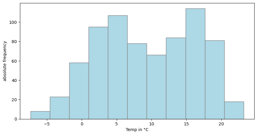
Ok, looks Bimodal! But there seems to be no normal distribution…..
2.3.5. Exercise 2C: Checking the mean and standard deviation for this subset#
Check for normality of the monthly mean temperature with the help of a qqplot!
### your code here ###
2.3.5.1. solution#
import statsmodels.api as sm

plt.figure(figsize=(12, 5))
sm.qqplot(dahlem_clim.MO_TT, line="r")

plt.show()
<Figure size 1200x500 with 0 Axes>
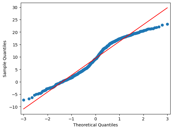
Well, we already suspected something like this…. Lets have a closer look:
2.3.6. Exercise 2D: Slicing the data frame#
Now, we want to slice the dataset into 2 parts. We want to subset between 1961 to 1990 and from 1991 to today. Subset the entire dataset (not only 1 column as we saw in the seminar)!
### your code here ###
2.3.6.1. solution#
## combined conditions :

dahlem_1961_1990 = dahlem_clim.loc[
    (dahlem_clim["MESS_DATUM_BEGINN"] >= 19610101)
    & (dahlem_clim["MESS_DATUM_BEGINN"] < 19910101)
]
dahlem_1961_1990
| STATIONS_ID | MESS_DATUM_BEGINN | MESS_DATUM_ENDE | QN_4 | MO_N | MO_TT | MO_TX | MO_TN | MO_FK | MX_TX | MX_FX | MX_TN | MO_SD_S | QN_6 | MO_RR | MX_RS | eor | |
|---|---|---|---|---|---|---|---|---|---|---|---|---|---|---|---|---|---|
| 2778 | 403 | 19610101 | 19610131 | 5 | 5.01 | -1.02 | 1.31 | -3.88 | 2.63 | 7.8 | -999.0 | -16.2 | 71.5 | 5 | 50.4 | 7.4 | eor |
| 2779 | 403 | 19610201 | 19610228 | 5 | 6.12 | 4.66 | 7.98 | 1.56 | 2.56 | 15.5 | -999.0 | -4.7 | 61.4 | 5 | 41.9 | 7.6 | eor |
| 2780 | 403 | 19610301 | 19610331 | 5 | 5.58 | 6.79 | 10.79 | 3.15 | 3.02 | 19.4 | -999.0 | -3.7 | 124.1 | 5 | 52.9 | 18.6 | eor |
| 2781 | 403 | 19610401 | 19610430 | 5 | 4.88 | 11.38 | 16.61 | 6.24 | 2.40 | 26.1 | -999.0 | -0.9 | 192.7 | 5 | 55.7 | 13.3 | eor |
| 2782 | 403 | 19610501 | 19610531 | 5 | 6.11 | 11.23 | 15.54 | 7.18 | 2.29 | 23.8 | -999.0 | 3.0 | 132.8 | 5 | 120.1 | 26.7 | eor |
| ... | ... | ... | ... | ... | ... | ... | ... | ... | ... | ... | ... | ... | ... | ... | ... | ... | ... |
| 3133 | 403 | 19900801 | 19900831 | 10 | 4.05 | 18.75 | 24.83 | 13.61 | 1.80 | 32.0 | 17.4 | 7.5 | 253.7 | 10 | 74.7 | 25.2 | eor |
| 3134 | 403 | 19900901 | 19900930 | 10 | 5.79 | 12.27 | 16.55 | 9.25 | 2.13 | 21.7 | 23.1 | 4.8 | 114.0 | 10 | 52.4 | 8.6 | eor |
| 3135 | 403 | 19901001 | 19901031 | 10 | 4.10 | 10.52 | 15.35 | 6.74 | 2.18 | 23.1 | 16.9 | 0.3 | 157.7 | 10 | 9.8 | 4.3 | eor |
| 3136 | 403 | 19901101 | 19901130 | 10 | 6.55 | 5.26 | 7.40 | 3.16 | 2.01 | 12.1 | 18.0 | -2.4 | 47.3 | 10 | 56.6 | 16.4 | eor |
| 3137 | 403 | 19901201 | 19901231 | 10 | 6.04 | 1.13 | 2.84 | -1.07 | 2.19 | 9.0 | 21.0 | -5.8 | 41.2 | 10 | 73.0 | 23.3 | eor |
360 rows × 17 columns
## combined conditions:

dahlem_1990_today = dahlem_clim.loc[dahlem_clim["MESS_DATUM_BEGINN"] >= 19910101]
dahlem_1990_today
| STATIONS_ID | MESS_DATUM_BEGINN | MESS_DATUM_ENDE | QN_4 | MO_N | MO_TT | MO_TX | MO_TN | MO_FK | MX_TX | MX_FX | MX_TN | MO_SD_S | QN_6 | MO_RR | MX_RS | eor | |
|---|---|---|---|---|---|---|---|---|---|---|---|---|---|---|---|---|---|
| 3138 | 403 | 19910101 | 19910131 | 10 | 4.97 | 2.30 | 4.57 | 0.07 | 2.16 | 15.2 | 18.5 | -8.7 | 76.20 | 9 | 27.6 | 13.7 | eor |
| 3139 | 403 | 19910201 | 19910228 | 10 | 5.27 | -2.34 | 0.85 | -5.32 | 1.84 | 12.9 | 14.9 | -12.9 | 72.40 | 9 | 27.1 | 7.9 | eor |
| 3140 | 403 | 19910301 | 19910331 | 10 | 4.79 | 6.77 | 11.30 | 3.25 | 2.15 | 18.1 | 14.4 | -1.2 | 128.30 | 9 | 40.8 | 19.0 | eor |
| 3141 | 403 | 19910401 | 19910430 | 10 | 4.80 | 8.23 | 13.28 | 3.32 | 2.02 | 20.5 | 20.0 | -2.8 | 174.80 | 9 | 40.4 | 7.8 | eor |
| 3142 | 403 | 19910501 | 19910531 | 10 | 4.97 | 10.52 | 14.90 | 5.90 | 2.19 | 24.2 | 24.1 | 1.2 | 179.60 | 9 | 38.6 | 15.5 | eor |
| ... | ... | ... | ... | ... | ... | ... | ... | ... | ... | ... | ... | ... | ... | ... | ... | ... | ... |
| 3505 | 403 | 20210801 | 20210831 | 3 | 5.67 | 17.43 | 22.34 | 12.97 | 2.42 | 29.4 | 16.9 | 8.0 | 188.23 | 3 | 92.4 | 22.6 | eor |
| 3506 | 403 | 20210901 | 20210930 | 3 | 4.90 | 15.55 | 20.28 | 11.35 | 2.33 | 27.3 | 18.6 | 6.8 | 154.48 | 3 | 35.1 | 15.9 | eor |
| 3507 | 403 | 20211001 | 20211031 | 3 | 4.85 | 10.49 | 15.28 | 6.29 | 2.81 | 24.2 | 25.6 | 0.5 | 157.65 | 3 | 21.8 | 5.7 | eor |
| 3508 | 403 | 20211101 | 20211130 | 3 | 6.65 | 6.28 | 8.68 | 3.87 | 2.60 | 12.7 | 18.6 | -0.9 | 41.23 | 3 | 65.2 | 40.4 | eor |
| 3509 | 403 | 20211201 | 20211231 | 1 | 6.57 | 2.19 | 4.30 | -0.11 | 2.74 | 14.0 | 21.5 | -10.2 | 38.18 | 3 | 39.2 | 8.8 | eor |
372 rows × 17 columns
2.3.7. Exercise 2E: Checking for Normality#
Calculate the mean and standard deviation for the monthly mean temperature for both dataframes! Doe they violate the three sigma rule? plot the distriubtion as histogram and density plot. Check for normality of the monthly mean temperature with the help of a qqplot! (solution the same as above)
### your code here ###
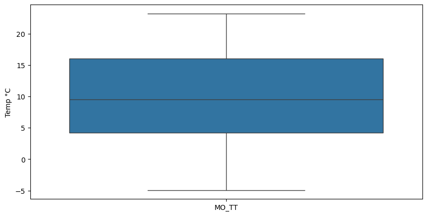
2.3.8. Exercise 2F: Boxplots#
Let’s have a closer look at both dataframes with the help of a boxplot! Plot both datasets next to eachother in two boxplots but one figure frame.
### your code here ###
2.3.8.1. solution#
fig = plt.figure(figsize=(10, 5))

sns.boxplot(data=[dahlem_1961_1990["MO_TT"], dahlem_1990_today["MO_TT"]])

plt.ylabel("Temp °C")
plt.show()
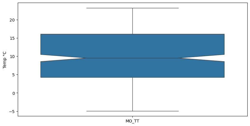
2.3.9. Exercise 2G: Nodges#
Which argument to we have to add, if we want to find significant differences between the groups? Is there a signifanct difference in the monthly mean temperature between 1961 to 1991 and from 1991 to today?
### your code here ###
2.3.9.1. solution#
fig = plt.figure(figsize=(10, 5))

sns.boxplot(data=[dahlem_1961_1990["MO_TT"], dahlem_1990_today["MO_TT"]], notch=True)

plt.ylabel("Temp °C")
plt.show()
from IPython.display import IFrame

IFrame(
    src="../../citations/citation_Marie.html",
    width=900,
    height=200,
)