3. Feature Scales#
3.1. Introduction to Empirical modelling#
What is a good model?
How to set up a good model?
How to decide if a published model is potentially valid?
Nice Introductory Video !!
3.1.1. Understanding the Problem#
almost all geoscientific characteristics are limited in scale space
statistics can estimate unknown (value) limits from observations
algebraic limits must be observed:
variable transformations must be carried out for certain calculations! Observing algebraic restrictions makes sense in terms of content!
The absolute majority of statistical methods is designed for unlimited rational (ℚ) or real feature scales (ℝ), thus any number between −∞ and +∞ are generally possible. We are expecting meaningful algebraic operations and ideally symmetric or better normal populations.
But nearly all variables are at least one-sided limited to the positive branch of ℝ or ℚ. Hereby, zeros are mostly meaningless and nearly always represent missing values. From an algebraic point of view only multiplication/division cannot leave the feature scale and mislead to estimate insufficient statistical parameters such as arithmetic mean or variances.
A closer look often reveals an additional upper limit of our variables space, mostly related to the physical frame of our planets gravity field and/or limited resources, ecological constraints and other reasons (distances, heights, temperature, counts of individuals, areas, brightness values, etc.). Furthermore, relative amounts or compositions are leading to spurious and sometimes crazy correlations or artificial patterns.
Therefore we have to “open” our bounded scales in order to perform mathematical/statistical right and meaningful results with regards to scientific contents. Many transformation are proposed in terms of achieving normality or symmetry. Some of them only change the shapes of distributions whereas other are solving algebraic constraints. Here, we are presenting linear and non-linear transformation as well as transformation for double constraint feature scales of compositional or physical nature.
(Nearly) all variables in Geosciences are limited to positive numbers!!!
3.2. Introduction to Model Sesign#
Basic principles: Mathematics, Physics & Statistics
Model design: Requirements, Recipe & Testing of existing models
scale of measurement! –> The guiding principle: design models in the real space!
3.2.1. Mathematics – spaces#
Space |
Notation |
Description |
Characteristics |
Examples |
|---|---|---|---|---|
Real Space |
\({\rm I\!R}\) |
interval scale |
\([-\infty, +\infty\)] |
time & space (location), e.g. UTM coordinates, changing the point of reference does not affect the pattern of the data. |
Positive Real Space |
\({\rm I\!R^+}\) |
ratio scale |
\(]0, +\infty]\) |
most physical quantities, e.g. temperature expressed in K (Kelvin), distance, time span, speed, permeability, and discharge.There is no origin on this scale: zero is a limiting value. |
Simplex |
\(S\) |
compositional scale |
\(]0,1[\) |
Sum must equal a constant (1 for proportions, 100 for percentages, \(10^6\) for ppm, e.g. concentrations, mass/ volume fractions |
3.2.2. Feature scales and machine learning approaches#
This is by no means a new idea !
Ada (Byron) Lovelace (letter to A. de Morgan 1840):
“I may remark that the curious transformations many formulae can undergo, the unsuspected and to a beginner apparently impossible identity of forms exceedingly dissimilar at first sight, is I think one of the chief difficulties in […]mathematical studies.
I am often reminded of certain sprites and fairies one reads of, who are at one’s elbows in one shape now, and the next minute in a form most dissimilar.”
(see Toole, B.A., 1998. Ada, the Enchantress of Numbers: Prophet of the Computer Age, Strawberry Press, ISBN 0912647183. p. 99)
As discussed above, normalization, scaling, standardization and transformations are crucial requirements for reliable and robust application of statistical methods beyond simple data description for getting meaningful results. Especially application of complex machine learning algorithms for exploration of multivariate data patterns it often becomes likely to get entrapped for violation of important preconditions. Hereby, it can be the violation of scale homogeneity using gradient descent related optimization technics or non-euclidean feature space for distance or angle related technics as well as simple violation of algebraic constraints.
A brief overview of common risk concerning serious pitfall is provided by Minkyung Kang in his data science blog:
3.2.2.1. ML Models sensitive to feature scale#
Algorithms that use gradient descent as an optimization technique
Linear Regression
Neural Networks
Distance-based algorithms
Support Vector Machines
KNN
K-means clustering Algorithms using directions of maximized variances
PCA / SVD
LDA
3.2.2.2. ML models not sensitive to feature scale#
Tree-based algorithms
Decision Tree
Random Forest
Gradient Boosted Trees
3.3. Reasons for transformations#
There are nearly unlimited reasons for scale transformation. Just to name a few, we focus on the following:
Scale homogeneity (e.g. different units, physical restriction)
Algebraic constraints on positive feature scales
Skewness, symmetry and normality
Double constraint feature scales
Compositional data sets
3.3.1. Algebraic constraints on limited feature scales#
Most real-world variables can only be positive (e.g. \(\mathbb{R_+}\) or \(]0,+\infty]\) or are limited to an interval (\(]a,b[_\mathbb{R_+}\)). Exceeding these boundaries by algebraic operations such as (+,-,*,/) leads to useless or meaning less results.
Example
On the scale of positive real numbers \(\mathbb{R_+}\) multiplication and the inverse operation division can not leave the set of positive real numbers. Thus, the positive real numbers together with the multiplication, denoted by \((\mathbb{R_+},*)\), form a commutative group with 1 as neutral element. In contrast, the set of positive real numbers together with the addition \((\mathbb{R_+},+)\) has neither inverse elements nor a neutral element. Thus, addition and subtraction can not be unlimited performed. But a log-transformation of any variable $\(x\in\mathbb{R_+}: x\to x'=\log(x)\)\( opens the scale to \)x’\to\mathbb{R}\( and transforms the neutral element of \)(\mathbb{R_+},\cdot)\( given by 1 to the neutral element of \)(\mathbb{R},+)\(, given by 0! The field of \)(\mathbb{R},+,\cdot)\( provides nearly unlimited operations for statistical purposes (except e.g. \)\sqrt{-1}\( or \)\frac{1}{0}$).
The inverse transformation powering $$x'\to x=e^{x'}$$
reverse the log-transformation back to the positive reel scale.
3.3.2. Skewness, symmetry and normality#
One reason for right skewed distributions can be the Hoelder inequality $\(\bar{x}_{geo}\leq \bar{x}_{arith}\)$ , but is not sufficient as explanation. Let us recall the geometric mean:
The main apparent difference between these two means is the operator: sum for arithmetic mean and product for the geometric mean. Thus, the arithmetic mean recommend for an additive or distance scale and the geometric mean for a ratio scale approach. In our case, we are dealing with a variable clearly hosted on the R+-scale where only multiplication is unlimited allowed.
But we often need an arithmetic mean for further statistical parameters: e.g.
standard deviation
skewness
covariance
correlation
regression
etc.
To solve this problem, we can apply the logarithm to the geometric mean:
3.3.2.1. Example: Working with a Dataset#
We begin by loading the meteorological data set from the Deutscher Wetterdienst DWD (German Weather Service) Open Climate Data Center . You find a documentation of this data in german and english.
Exercise:
Calculate standard deviation and arith. Mean of the monthly sum of precipitaiton height!
Check the 3-sigma rule and plot the distribution!
# First, let's import all the needed libraries.
import numpy as np
import pandas as pd
import matplotlib.pyplot as plt
import scipy.stats as stats
import seaborn as sns
import statsmodels.api as sm
# read dataset from online ressource
dahlem_clim = pd.read_csv(
    "https://userpage.fu-berlin.de/soga/data/raw-data/NS_TS_Dahlem.txt", sep=";"
)
dahlem_clim.head(10)  # display first 10 entries
| STATIONS_ID | MESS_DATUM_BEGINN | MESS_DATUM_ENDE | QN_4 | MO_N | MO_TT | MO_TX | MO_TN | MO_FK | MX_TX | MX_FX | MX_TN | MO_SD_S | QN_6 | MO_RR | MX_RS | eor | |
|---|---|---|---|---|---|---|---|---|---|---|---|---|---|---|---|---|---|
| 0 | 403 | 17190101 | 17190131 | 5 | -999.0 | 2.8 | -999.0 | -999.0 | -999.0 | -999.0 | -999.0 | -999.0 | -999.0 | -999 | -999.0 | -999.0 | eor |
| 1 | 403 | 17190201 | 17190228 | 5 | -999.0 | 1.1 | -999.0 | -999.0 | -999.0 | -999.0 | -999.0 | -999.0 | -999.0 | -999 | -999.0 | -999.0 | eor |
| 2 | 403 | 17190301 | 17190331 | 5 | -999.0 | 5.2 | -999.0 | -999.0 | -999.0 | -999.0 | -999.0 | -999.0 | -999.0 | -999 | -999.0 | -999.0 | eor |
| 3 | 403 | 17190401 | 17190430 | 5 | -999.0 | 9.0 | -999.0 | -999.0 | -999.0 | -999.0 | -999.0 | -999.0 | -999.0 | -999 | -999.0 | -999.0 | eor |
| 4 | 403 | 17190501 | 17190531 | 5 | -999.0 | 15.1 | -999.0 | -999.0 | -999.0 | -999.0 | -999.0 | -999.0 | -999.0 | -999 | -999.0 | -999.0 | eor |
| 5 | 403 | 17190601 | 17190630 | 5 | -999.0 | 19.0 | -999.0 | -999.0 | -999.0 | -999.0 | -999.0 | -999.0 | -999.0 | -999 | -999.0 | -999.0 | eor |
| 6 | 403 | 17190701 | 17190731 | 5 | -999.0 | 21.4 | -999.0 | -999.0 | -999.0 | -999.0 | -999.0 | -999.0 | -999.0 | -999 | -999.0 | -999.0 | eor |
| 7 | 403 | 17190801 | 17190831 | 5 | -999.0 | 18.8 | -999.0 | -999.0 | -999.0 | -999.0 | -999.0 | -999.0 | -999.0 | -999 | -999.0 | -999.0 | eor |
| 8 | 403 | 17190901 | 17190930 | 5 | -999.0 | 13.9 | -999.0 | -999.0 | -999.0 | -999.0 | -999.0 | -999.0 | -999.0 | -999 | -999.0 | -999.0 | eor |
| 9 | 403 | 17191001 | 17191031 | 5 | -999.0 | 9.0 | -999.0 | -999.0 | -999.0 | -999.0 | -999.0 | -999.0 | -999.0 | -999 | -999.0 | -999.0 | eor |
Dahlem_NS = dahlem_clim.MO_RR[2767:3510] # subset precip. MO_RR, starting 1961
3.3.2.1.1. solution#
np.mean(Dahlem_NS)
48.7950201884253
np.std(Dahlem_NS)
29.251147878103385
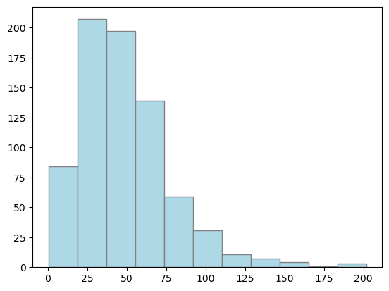
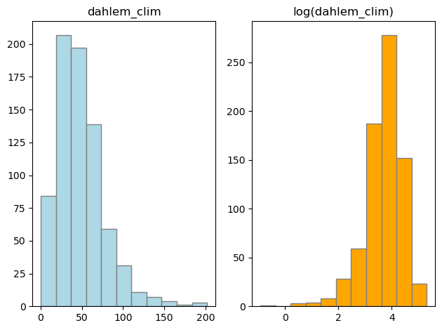
plt.hist(Dahlem_NS, bins="sturges", color="lightblue", edgecolor="grey")
plt.show()
3.3.2.2. Exercise:#
Calculate the mean and standard deviation of the logarithmised values and transform them back!
Calculate the limits of the 3-sigma rule in the same way!
#### your code here ####
3.3.2.2.1. solution#
np.exp(np.mean(np.log(Dahlem_NS)))
39.87362261019636
np.exp(np.std(np.log(Dahlem_NS)))
2.040964347643825
fig, axs = plt.subplots(1, 2)


axs[0].hist(Dahlem_NS, bins="sturges", color="lightblue", edgecolor="grey")
axs[0].set_title("dahlem_clim")
axs[1].hist(np.log(Dahlem_NS), bins="sturges", color="orange", edgecolor="grey")
axs[1].set_title("log(dahlem_clim)")


# for ax in axs.flat:
#   ax.set(xlabel='x-label', ylabel='y-label')

# Hide x labels and tick labels for top plots and y ticks for right plots.
# for ax in axs.flat:
#    ax.label_outer()
plt.tight_layout()
plt.show()
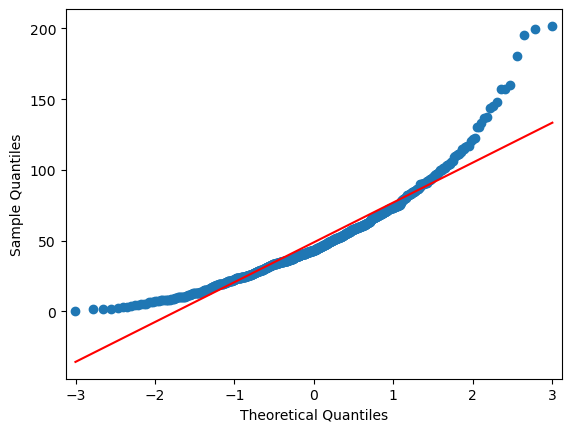
import statsmodels.api as sm
plt.figure(figsize=(12, 5))
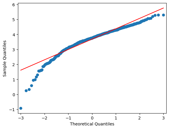
sm.qqplot(Dahlem_NS, line="r")
plt.show()
<Figure size 1200x500 with 0 Axes>
import statsmodels.api as sm

plt.figure(figsize=(12, 5))
sm.qqplot(np.log(Dahlem_NS), line="r")

plt.show()
<Figure size 1200x500 with 0 Axes>
3.3.3. Double constrained feature spaces#
There is a certain relation to the compositional constraint if we face double bounded feature spaces. Let us imagine a variable $\mathbf{x}=(x_i\in ]l,u[_\mathbb R,i=1,\cdots,m)$ within a constrained interval [a,b]$\subset \mathbb R$. The absolute value is obviously of minor interest compared with the relative position between l and u. A first step should be a linear min-max-transformation wit min=l and max=u:
$$ x \to x' =\frac{x-l}{u-l} \in\ ]0,1[\ \in \ {\mathbb R}_+ $$Now, x' divides the interval into two parts: 1. the distance to the left (=x) and 2. the distance to the right (1-x). Both sum up to 1 and are therefore related to a 2-dimensional composition.
In Application, the formula should look like this:
Applying an alr-transformation to our variable, we are getting a symmetric feature scale: $\( x'\to x''=\log(\frac{x'}{1-x'})\in \mathbb R\)\( This so-called <em>logistic transformation</em> enable application of algebraic operation over the base field \)\mathbb R$.
The back transformations are:
The back transformation is the “logistic” function resp. inverse logit:
3.3.3.1. Example: Northern hemispheric ice extent under climate change#
The National Snow and Ice Data Center at the University of Colorado in Boulder hosts and provides monthly sea ice data for both hemispheres since November 1978 to present. Under the condition of a warming earth system, we will estimate the changes for the northern hemisphere and project a possible trend until the end of this century for September.
Step 1: Loading the data and plotting the time series
# open the data set as csv file using pandas

df = pd.read_csv(
    "ftp://sidads.colorado.edu/DATASETS/NOAA/G02135//north/monthly/data/N_09_extent_v3.0.csv",
    skipinitialspace=True,
)
df.head()
| year | mo | data-type | region | extent | area | |
|---|---|---|---|---|---|---|
| 0 | 1979 | 9 | Goddard | N | 7.05 | 4.58 |
| 1 | 1980 | 9 | Goddard | N | 7.67 | 4.87 |
| 2 | 1981 | 9 | Goddard | N | 7.14 | 4.44 |
| 3 | 1982 | 9 | Goddard | N | 7.30 | 4.43 |
| 4 | 1983 | 9 | Goddard | N | 7.39 | 4.70 |
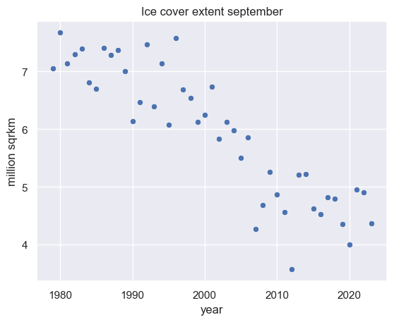
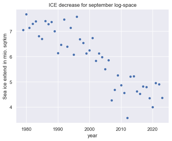
# use seaborn for plotting

sns.set()

sns.scatterplot(data=df, x="year", y="extent")
plt.title("Ice cover extent september")
plt.ylabel("million sqrkm")
Text(0, 0.5, 'million sqrkm')
Step 2: Prediction
Now, we may estimate the linear trend using seeborn.regplot. If we set ‘truncate = True’ regression line is bounded by the data limits. If we set ‘truncate = False’, it extends to the x axis limits.
plt.xlim(1975, 2100)
plt.ylim(0, 10)
sns.regplot(data=df, x="year", y="extent", truncate=False, ci=95)
plt.title("Prediction of the ice cover extent september")
plt.ylabel("million sqrkm")
Text(0, 0.5, 'million sqrkm')
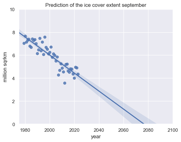
Modeling the observed ice cover extent from 1979 to 2020 for the northern hemisphere in September for the future, we have to expect a complete disappearance of the arctic ice in late summer with 95% probability within the second half of this century!
In 2035 we may expect an ICE in september with 95% confidence level between 2.07 and 4.41 milion sqrkm, therefore between 51.83% and 110.3% of last september extent.
In 2050 we may expect an ICE in September with 95% confidence level between 0.8 and 3.31 milion sqrkm, therefore between 20.09% and 82.77% of last september extent.
The feature scale of the arctic ice extent in million square kilometer is clearly framed by a lower and upper limit: The extent definitly can neither be negative nor pass the equator. Thus, the lower limit is trivial but the upper limit unknown.
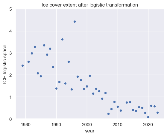
For the sake of simplicity we initially use the maximum extent as upper limit and remove this maximum from our time series and start a logistic approach:
Step 3: Logistic Transformation
We start by scaling the data to the standard simplex ]0,1[ℝ+ by deviding the data by the maximum as estimate of the upper limit. Afterward we transform the standard simplex by logistic transformation and plot the transfomed time series.
df["extent lrt"] = df["extent"] / max(df["extent"])

# if we hit the maximum, the outcome is 1. For this value, we can not calculate the logarithm. Therefore, we need
# to exclude the value or approximate it by, e.g. 0.999999:

for i in range(0, len(df["extent lrt"])):

    if df.iloc[i, 6] == 1:
        df.iloc[i, 6] = 0.999999


df["extent lrt"] = np.log(df["extent lrt"] / (1 - df["extent lrt"]))
## Plot the data:

sns.scatterplot(data=df, x="year", y="extent lrt")
plt.title("Ice cover extent after logistic transformation")
plt.ylim(0, 5)
plt.ylabel("ICE logistic space")
Text(0, 0.5, 'ICE logistic space')
Step 4: Estimating the trend
Now, we can fit a linear model in the log-space:
plt.xlim(1977, 2100)
plt.ylim(-6, 5)
plot_des = sns.regplot(data=df, x="year", y="extent lrt", truncate=False)
plt.axhline(0)
plt.title("Prediction of ICE decrease for september log-space")
plt.ylabel("ICE logistic space")
Text(0, 0.5, 'ICE logistic space')
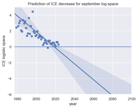
Interpreting the zero base of the upper plot, half of the former ice cover extent (expressed by the maximum of observation) has dissapeared since roughly 2010.
Back transformation in the original space:
Next, let us us transform the model in the original space by
# Since sns.regplot does not provide the coefficients of the regression line, we calculate the
# coefficients by statmodels. Both approaches calculate the parameters analogously, so we may do this.


y = df.iloc[:, 6]
x = df.iloc[:, 0]
x = sm.add_constant(x)
alpha = 0.05  # 95% confidence interval
model = sm.OLS(y, x)
lr = model.fit()
# lr = sm.OLS(y, sm.add_constant(x)).fit()
# print(lr.params)

print(lr.summary())

# Slope: a
a = lr.params[1]

# Intercept: b
b = lr.params[0]

# Confidence intervals:
lr_ci = lr.conf_int(alpha=0.05)

# enlarge data until the year 2100:
x_1979_2100 = pd.DataFrame(np.arange(1979, 2100), columns=["year"])
# x_test = [1] * len(x_1979_2100)
x_1979_2100 = sm.add_constant(x_1979_2100)

y_1979_2100 = lr.predict(x_1979_2100)
                            OLS Regression Results
==============================================================================
Dep. Variable:             extent lrt   R-squared:                       0.381
Model:                            OLS   Adj. R-squared:                  0.366
Method:                 Least Squares   F-statistic:                     26.42
Date:                Fri, 19 Jul 2024   Prob (F-statistic):           6.40e-06
Time:                        12:32:25   Log-Likelihood:                -86.781
No. Observations:                  45   AIC:                             177.6
Df Residuals:                      43   BIC:                             181.2
Df Model:                           1
Covariance Type:            nonrobust
==============================================================================
                 coef    std err          t      P>|t|      [0.025      0.975]
------------------------------------------------------------------------------
const        202.7756     39.110      5.185      0.000     123.902     281.649
year          -0.1005      0.020     -5.140      0.000      -0.140      -0.061
==============================================================================
Omnibus:                       81.579   Durbin-Watson:                   2.337
Prob(Omnibus):                  0.000   Jarque-Bera (JB):             1377.022
Skew:                           4.699   Prob(JB):                    9.63e-300
Kurtosis:                      28.418   Cond. No.                     3.08e+05
==============================================================================

Notes:
[1] Standard Errors assume that the covariance matrix of the errors is correctly specified.
[2] The condition number is large, 3.08e+05. This might indicate that there are
strong multicollinearity or other numerical problems.
/var/folders/vs/k3tcf9r11xq5pqzsg6kq3sx00000gn/T/ipykernel_54646/3064685890.py:17: FutureWarning: Series.__getitem__ treating keys as positions is deprecated. In a future version, integer keys will always be treated as labels (consistent with DataFrame behavior). To access a value by position, use `ser.iloc[pos]`
  a = lr.params[1]
/var/folders/vs/k3tcf9r11xq5pqzsg6kq3sx00000gn/T/ipykernel_54646/3064685890.py:20: FutureWarning: Series.__getitem__ treating keys as positions is deprecated. In a future version, integer keys will always be treated as labels (consistent with DataFrame behavior). To access a value by position, use `ser.iloc[pos]`
  b = lr.params[0]
df["extent back trafo"] = (
    (np.exp(df["extent lrt"])) / (1 + (np.exp(df["extent lrt"]))) * df["extent"].max()
)
# predict until 2021:

lr_back = (
    (np.exp(a * x_1979_2100.iloc[:, 1] + b))
    / (1 + (np.exp(a * x_1979_2100.iloc[:, 1] + b)))
) * df["extent"].max()
x_1979_2100.iloc[:, 1]
0      1979
1      1980
2      1981
3      1982
4      1983
       ...
116    2095
117    2096
118    2097
119    2098
120    2099
Name: year, Length: 121, dtype: int64
Let us have a look on the scatter plot of the transformed data:
sns.scatterplot(data=df, x="year", y="extent back trafo")
plt.title("ICE decrease for september log-space")
plt.ylabel("Sea ice extend in mio. sqrkm")
Text(0, 0.5, 'Sea ice extend in mio. sqrkm')
Estimating the trend:
# In order to plot the logistic regresion line (orange line below, we create a new data set with the back transformed data
# of the linear regression line

d_1979_2100 = {"year": np.array(x_1979_2100)[:, 1], "extent": lr_back}
df_1979_2100 = pd.DataFrame(data=d_1979_2100)
plt.xlim(1977, 2100)
plot_des = sns.regplot(data=df, x="year", y="extent back trafo", truncate=False)
plt.axhline(0)
plt.axhline(1)
plt.title("Prediction of ICE decrease for september log-space")
plt.ylabel("ICE logistic space")

sns.lineplot(data=df_1979_2100, x="year", y="extent")
<Axes: title={'center': 'Prediction of ICE decrease for september log-space'}, xlabel='year', ylabel='ICE logistic space'>
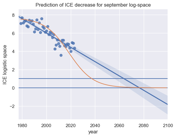
As an exercise, you can transform the confidence intervals of the regression line in the log space and you will get the following result:
With 95% probability, the arctic ice extent may pass the 1-million sqrkm marker between 2030 and 2070 and a complete disappearance in the second half of our century. This simple empirical estimation is able to confirm the sophisticated physical modeling approach by Peng et al. 2020.
3.3.4. Compositional contraints#
Compositional data is a special type of of non-negative data, which carries the relevant information in the ratios between the variables rather than in the actual data values. The individual parts of the composition are called components or parts. Each component has an amount, representing its importance within the whole. The sum over the amounts of all components is called the total amount, and portions are the individual amounts divided by this total amount (van den Boogaart and Tolosana-Delgado 2013).
Compositions are sets of variables which values sum up to a constant, e.g.
dissolved cations and anions in a liquid
frequencies of population groups (e.g. employees, jobless people, etc.)
role allocation of a person during a time span in behavioral sciences
nutrition content for food declaration
many, many more …
The great challenge of compositional data is that no single component can be regarded as independent from other. This means, if you observe a (e.g. spatial or temporal) pattern within one single component, at least parts of the pattern is likely rather attributed to another part of the composition than the (spatial or temporal) behaviour of the varibale of interest it self. Due to the compositional nature of such variable, they can neither be independent nor normal.
A simple example:

Imagine two measurements of a 2-part composition which sum up to a whole: Within measurement 1, both parts are uniform with exact 50% of the whole composition. Measurement 2 is showing up with 70% of the dark gray component and 30% the light grey one. How can we describe the difference: Has the dark grey component increased whereas the light grey remained constant or has the light grey component decreased and the dark grey remained constant? It is absolutely impossible to decide what has happened, because both cases would show up with a similar pattern. Furthermore, we have to consider that all values are strictly positive and thus, differences are rather related to ratios than for distances.
Hence, 40% of the lightgrey part has been shifted to the dark grey, but we still cannot decide whether x increased or y decreased.
What does this imply beside spurious correlations?
We can interpret the correlation coefficient as normalized cosine of the angle between the deviation vectors to the mean $$\mathbf{x}_{d}=(x_i-\bar{x},i=1,\cdots,n)$$
and
$$ \mathbf{y}_{d}=(y_i-\bar{y},i=1,\cdots,n)$$The cosine of the angle between two vectors is calculated by the scalar product divided to the product of both norm:
Setting $\mathbf{x} =\mathbf{x}-\overline{\mathbf{x}}$ and $\mathbf{y} =\mathbf{y}-\overline{\mathbf{y}}$, we are getting the scalar product as nominator for the covariance term and the product of the norms as standard deviation terms.
Thus, in compositions the deviations vectors as bases are oblique by nature and consequently non-euclidean!
Hence, statistical methods using distances and angles (ratios) as optimization parameters can not be applied on pure compositions. Such methods are e.g.:
- (ML-)regression and correlation, GLM, PCA, LDA, ANN
- SVM, KNN, k-Means
- most hypotheses tests, etc.
Whereas, this problem is well known since Karl Pearson published the problem of spurious correlation in compositional data 1897 more than 100 years ago Felix Chayes suggest the use of ratios instead of portions: $$ a,b \in ]0,1[_{\mathbb{R}}\to \frac{a}{b}\in \mathbb{R_+} $$ One of the remaining disadvantage was now the question about nominator and denominator, because of the often huge difference between a/b and b/a. Another problem was still the limit to the positive reel feature scale.
In 1981, the Scottish statistician John Aitchison solved the problem introducing the log-ratios: $$ \log \frac{a}{b}=-\log \frac{b}{a}\in\mathbb R\, .$$ Thus, changing nominator and denominator just change the sign of the log-ratio but not the absolute value implies symmetry again (cf. paragraph above) In his Book The statistical analysis of composional data, 1986 introduced
- Additive log-ratio (alr) transformation is the logarithm of the ratio of each variable divided by a selected variable of the composition. Alr applied on a D-dimensional composition results in a D-1-dimensional variable space over the field $(\mathbb{R},+,\cdot)$. Unfortunately, beside a asymmetry in the parts, alr is not isometric. Thus, distances and angles are not consistence between simplex and the resulting D-1 dimensional subspace of $\mathbb{R}^D$.
- Centered log-ratio (clr) transformation is the logarithm of the ratio of each value divided through the geometric mean of all parts of the corresponding observation. The clr transformation is symmetric with respect to the compositional parts and keeps the same number of components as the number of parts in the composition. Due to the problem that orthogonal references in that subspace are not obtained in a straightforward manner, Egozcue et al. 2003 introduced:
- Isometric log-ratio (ilr) transformation is isometric and provides an orthonormal basis. Thus, distances and angles are independent from the sub-composition (symmetric in all parts of the sub-composition) comparable between the Aitchison simplex and the D-dimensional reel space.
However, PCA or SVD-analysis on a clr-transformed simplex provides similar properties Egozcue et al. 2003.
In Python you may easily use the compostions.stats module for compostional constraints!
Learn more about clr, alr, ilr here!
from IPython.display import IFrame

IFrame(
    src="../../../citation_Soga.html",
    width=900,
    height=200,
)